I’ve discussed in the past how to indicate statistical significance with colour rather than stars. Another concern people have about using Beamer is that it can be hard to squish results into one slide. In my opinion, that is solved very easily with my tinytable command.

\documentclass[xcolor={table}]{beamer}
\usepackage{booktabs}

\newcommand{\tinytable}[1]{\textcolor{black}{\tiny \input{#1} }}

\begin{document}
\begin{frame}
\frametitle{Fascinating}
\input{myoutput}
\end{frame}

\begin{frame}
\frametitle{Still fascinating, but smaller}
\tinytable{myoutput}
\end{frame}
\end{document} 

This generates the following:

//

The economic package includes old commands that are now deprecated within LaTeX. This caused me a problem using the AER bibliography style (aer.bst), and likely causes problems with other BibTeX styles too. My particular problem was with scrartcl refusing to recognise the \bf command rather than the newer \textbf version.

Very specifically, the problem was “Class scrartcl Error: undefined old font command `\bf’.”

The fix for this is simple. Just include the following two lines in the preamble of your document.

\DeclareOldFontCommand{\bf}{\normalfontbfseries}{\textbf}
\DeclareOldFontCommand{\it}{\normalfont\itshape}{\textit}

You could alternatively open up your *.bst file and manually change the code, but the two lines above should fix it.

//

There has been much hand-wringing about Apple’s low effective tax rates, particularly since the European Commission’s declaration that they know more about the correct implementation of Ireland’s tax laws than Ireland’s own tax authorities. This has focused the public eye on the taxation of multinational corporations in Ireland and elsewhere. There is a problem with the taxation of MNCs, but I argue it is a problem largely attributable to actions in Washington DC, not anywhere else.


Let me explain. The US headline corporate tax rate is 35%. Thus if an American company earns $100 in the United States, the IRS expects that company to pay a total of $35 in taxes. Further, the US corporate tax base is structured on a worldwide income system. So if Starbucks earns $100 in Denmark, the IRS still expects the company to pay a total of $35 in taxes. For example, if Starbucks pays $20 in taxes to Denmark, the residual $15 is due in taxes to the US. (See here for an example of this offsetting rule.)

Continuing with the Denmark example, the amount due to the Danish government must by law account for the fact that a lot of Starbucks’ profitability comes from its intellectual property: its recipes, branding, and so on. That intellectual property is American, not Danish. For the sake of argument, let’s say that 75% of Starbucks’ profitability in Denmark is based on American intellectual property, and the rest is due to shrewd decisions by managers in Copenhagen. (Change these numbers as you see fit, the idea still holds.) Thus although Starbucks will technically book $100 of profit in Denmark, 75% of that is “American profit”, with only 25% attributable to decisions by the Danish operation. Denmark’s corporate tax rate is 22%, so Starbucks will owe 22% of $25 = $5.50 to Denmark. But recall that they booked $100 of gross profits in Denmark so, on the face of it, The Guardian and other such outlets will wail that Starbucks gets away with a tax rate of only 5.5%. How unfair, how unjust, etc.

Of course what The Guardian and The Huffington Post will typically fail to mention is that the IRS expects the residual $29.50 to be paid in the US ($35 less the $5.50 paid in Denmark = $29.50). That is the main reason why newspaper headlines mislead the public. But a further, more substantive issue that is rarely discussed in the media is where the real problem comes in: the United States’ unusual treatment of (unrepatriated) foreign profits.

What is this unusual treatment? Starbucks do not have to pay that tax liability until they redistribute the profits back to the shareholders by way of a dividend payment. So it is perfectly legal, as per the Tax Reform Act of 1986, for Starbucks’ profits to sit in a bank earning interest rather than paying up to the IRS.

Regular US taxpayers have to pay their previous year’s taxes by April 15th. Corporations can choose when they pay up, and they are welcome under US tax law to wait many years to do so. They may even hold out in the hope that Congress drops the tax rate — for example Donald Trump has proposed lowering the corporate tax rate from 35% to 15% — and end up paying much less than previously thought. Apple is sitting on about $150bn dollars of unrepatriated profits. They’re holding out (completely sensibly, from their perspective) for a law change so when it comes to paying up, they do so at a lower rate. This holding out again makes it appear that companies like Apple’s tax liabilities are lower than they actually are. How unfair, how unjust, etc. Yet I don’t think I have ever seen a newspaper discuss the intricacies of why an existing US law — the Tax Reform Act of 1986 — encourages this perverse behaviour, nor do I predict a flurry of articles heaping praise on Apple or Starbucks when their effective tax rate shoots through the roof when they eventually repatriate back-dated income.

You can also perhaps see why Apple’s low tax payments in Ireland are an issue for Washington, not Dublin.

Finally, all this is relatively moot if we fail to consider the incidence of corporate taxes. Most members of the public understand that taxes on oil are passed onto the consumer, at least in part. However, the same logic has yet to penetrate the public consciousness on corporate taxes. If you tax a corporation, the workers and customers of that corporation cannot magically wave a moral wand and avoid the economic repercussions of the tax. Some of that tax will inevitably be passed onto consumers, some onto workers, some onto shareholders, etc.

Exactly how the tax is split between groups is a tricky thing to statistically disentangle. However, recent research suggests that about 30% of corporate taxes in the US are passed onto the corporation’s employees; and excellent work by German economists suggests that over there perhaps as much as 80% is passed onto workers. The clamour for increased taxation of multinationals almost never considers this reality. I have never seen it mentioned in newspapers that if large multinationals are successfully dodging taxes, it is almost certain that their consumers and workers also benefit from this.

To be clear: I like The Guardian; the Tax Reform Act was a considerable improvement overall; and corporations should pay the tax rates that are demanded of them by law. However the depiction of corporate taxation in the media routinely overlooks mandatory deductions for intellectual property, the deferral of unrepatriated foreign earnings, and the crucial issue of incidence/who actually pays the corporate tax.

Debate on the topic suffers as a result.
//

I like being able to hide content in documents, for example including but not revealing the answers in a problem set. That makes it very easy to then produce the problem set solutions, simply by revealing the answers. I made this easier with a \hide{} command, that can be “turned off” so the answers are revealed.

This is the basic code I use for producing problem sets. The only change needed to convert a problem set into a solution set is to redefine the \showanswers variable to equal 1 rather than 0.

\documentclass{article}
% Set this =0 to hide, =1 to show
\def\showanswers{0}

\newcommand{\hide}[1]{
\ifnum\showanswers=1

#1 \vspace{\baselineskip}
\fi

\ifnum\showanswers=0

\vspace{2\baselineskip} \hspace{2cm}
\fi
}

\begin{document}

\begin{enumerate}
\item This is question 1.
\hide{Here is a hidden solution.}


\item What is the answer to question 2?
\hide{The answer is here.}
\end{enumerate}

\end{document}
//

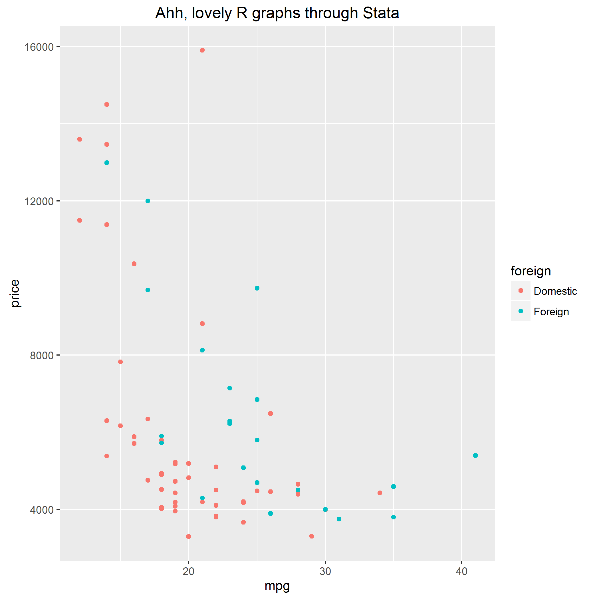
Stata is great, but it’s true that R makes prettier graphs, especially when you make use of the outstandingly excellent ggplot2 Thanks to Roger Newson we can have both. This post walks you through exploiting ggplot2 directly from Stata. I’ve tested this with both Stata 13 and Stata 14 on Windows 7 on two different computers.

A simple ggplot produced directly from Stata

Here are the steps:

  • First, you need the foreign and ggplot2 packages installed in R. Install them using the install.packages() command, e.g. install.packages("ggplot2")
  • Second, you need the rsource package installed in Stata. You can do this with the ssc inst rsource command.
  • Third, you need to find the R terminal program, named Rterm.exe. For me, this is located in C:/Program Files/R/R-3.3.0/bin/x64/Rterm.exe. You then need to change the line in the code that begins with global Rterm_path to wherever Rterm.exe is on your computer.

Then you can use this code (click here for download). It’s well commented below so you should be able to understand what it’s doing. It produces the graph you can see above.

** Open up R interactively through Stata
** Enda Patrick Hargaden
** Boyd Center / Economics
** University of Tennessee, July 2016

** For sample purposes, let's use the auto dataset. Obviously you change this to your data.
clear
sysuse auto

***********************************************
** You need to adjust this. Find the location of Rterm.exe on your machine
***********************************************
global Rterm_path `"C:/Program Files/R/R-3.3.0/bin/x64/Rterm.exe"'

** This records Stata's present working directory in R-compatible format
local r_pwd = subinstr("`c(pwd)'","","/",.)

** Temporarily make a copy of the dataset in a format R will probably understand
saveold holderfile.dta, version(12) replace

** Start R via rsource, pass your present working directory to it
rsource, terminator("end_r_stata") roptions(`" --vanilla --args "`r_pwd'" "')

## We're now in R, so switching the comment designation from star to hash
## Stata may mention an error anytime you include an R comment. Don't worry about it.

## Use the argument (i.e. pwd) passed via Stata and move to it
stata_pwd = commandArgs(trailingOnly=TRUE);
setwd(stata_pwd[1]);

## Load the packages.
library("foreign");
library("ggplot2");

## Read and then delete the data
df = read.dta("holderfile.dta", convert.f=TRUE)
file.remove("holderfile.dta")

## Draw the graph
ggplot(df, aes(x=mpg, y=price, color=foreign)) +
geom_point() +
ggtitle("Ahh, lovely R graphs through Stata")

## Save both a PDF and PNG version
ggsave("ggplot_stata.pdf")
ggsave("ggplot_stata.png")

## And now you stop using R
end_r_stata

And there we have it. Transferring the data over to R and generating nice ggplots without ever leaving Stata. Of course you don’t need to restrict yourself to ggplots. With this basic idea you can use any of R’s capabilities directly from Stata.

//

"The decisive inhibitions, then, will always be those on the actual use of nuclear weapons. By far the worst consequences of their possession would be the use of them. Possession itself can be mischievous; and the stronger the perceived limitations on the usefulness of nuclear weapons, the stronger will be the considerations militating against acquisition.

There is a stronger way to phrase this. A government that would use nuclear weapons if it had them, and could get them, would get them. No inhibition on mere possession could survive a decision to use them. [...]

In these conditions---and we are probably talking about the 1990s---possessing or not possessing some nuclear weapons, or having it known or not known that a country possesses some nuclear weapons, will not decisively differentiate countries as it may have done in the past. The difference will seem greatest when it doesn't matter much. [...]

The organizations most likely to engage in nuclear terrorism will be national governments. Passive terrorism on a grand scale we call "deterrence." When it is directed at us, rather than at our enemies, we call it "blackmail." [...]

Some of the more dramatic acts of terrorism that we have read about in recent years have been initiated by individuals or small groups that had more passion than perseverance, more interest in getting attention than in getting results. They did not appear to be well-articulated pieces of a grand strategy in furtherance of a major objective. Most of them do not seem to have involved careful planning by large numbers of thoughtful people. But an organization that had the brains and the money and the teamwork and the discipline to bring off the successful construction of a nuclear bomb would have plenty of time and plenty of reason to think carefully about how to use this potential influence, this dreadful threat that may be as diplomatically unwieldy as it is enormous."

-- Thomas Schelling (1984), "Who Will Have the Bomb?" in Choice and Consequence.

//

Michigan's Graduate Student Instructors (GSIs) receive student evaluations for every class they teach. The undergrads are invited to rate their GSIs using Likert Scales (aside: Likert had a degree in economics from the University of Michigan). Students see something like this:

Overall, the instructor was an excellent teacher
Strongly Disgree Disagree Neutral Agree Strongly Agree

The Registrar compiles this data, encoding "Strongly Disagree" as 1, "Strongly Agree" as 5, etc. They then provide GSIs with what is called their "Median score", which is actually a slightly complicated interpolated form of the median.

The application of medians to discrete values was perplexing, so I asked the Office of the Registrar to provide me with the exact formula they use. They did so, and I reproduce it here in case any GSI in the future ever wonders as I once did. (I checked: the Registrar has no objection to this being made public knowledge.)

Their formula, which requires some lingo that is explained below, is:

\(\text{Median } = \text{Lower Real Limit } + \frac{0.5N - a}{b}\)

Calculate the range the median must lie in, e.g. somewhere between 2 and 3. Let's call this range "the interval". The Lower Real Limit is the midway point of the interval, i.e. 2.5.

The total number of observations (in the whole sample) is denoted \(N\). Denote as \(a\) the number of responses below the Lower Real Limit. In this example, \(a\) would be equal to the numbers of 1s and 2s.

Recall that our interval is the range between 2 and 3. The upper-limit of this is 3. Finally, denote as \(b\) the number of observations that choose the upper-limit of this interval, i.e. the number of people that chose 3.

Now for an example, suppose you have the following scores:

Score 1 2 3 4 5
Frequency 2 1 8 14 7

By inspection, the median cannot be greater than 4 and cannot be lower than 3. Therefore our interval is 3-4, with a Lower Real Limit of 3.5. There are 32 responses, so \(N=32\). Eleven people chose a score below the Lower Real Limit, so \(a=11\). Fourteen people chose the upper-limit of the interval, so \(b=14\). Plugging this into our equation above:

\(\text{Median } = 3.5 + \frac{0.5(32) - 11}{14} = 3.86\).

//

While watching football this morning, I also kept an eye on the betting odds. As soon one team scored, the odds changed.

Instead of introducing the efficient market hypothesis to students as a theory about stocks and bonds, we should perhaps start by drawing parallels to sports-betting. It is hard to consistently make money betting on Premier League results. It's not impossible, but it takes a lot of skill and/or luck to pull it off.

The same logic applies to beating the general rate of return in a market. Financial markets tend to adjust prices so that there are no obvious bargains. This is not a claim that sporting events never throw up shock victories, nor does it imply that markets never crash. If anything, it suggests that predicting a stock market crash is about as difficult as predicting a shock sporting victory.

Like comparative advantage, it's hard for undergrads to grasp this idea. I have found that the sporting analogy works well as a stepping stone.

(While on the topic of the EMH: there's a fun contrast between the predicament of Cassandra, who could perfectly predict the future but nobody would believe her, and the EMH. The more people believe in EMH, the less likely they are to actively search for arbitrage opportunities. This will tend to leave market-beating returns uncollected, nullifying the EMH. The converse also holds. In this respect, EMH is a self-defeating prophecy.)

//
Scroll to Top